[19]:
WORKDIR=%pwd
Example 2: Water dipole and polarizability
Tasks
Train dipole and polarizability of bulk water.
Use LAMMPS Calculator interface.
Plot the infrared and raman spectrum.
Prepare data
You can see the following files required by training in this fold.
water
|- dipole.yaml
|- polar.yaml
|- data/
   |- train.xyz
   |- test.xyz
`dipole.yaml <dipole.yaml>`__ and `polar.yaml <polar.yaml>`__ controls the details of model architecture and training for dipole and polarizability respectively. Some import parameters in this tasks are:
For dipole.yaml:
cutoff: 4.0
Data:
  trainSet: data/train.xyz
  testSet: data/test.xyz
Train:
  targetProp: ["dipole"]
  weight: [1.0]
These parameters mean the cutoff in this task is 4.0 Å. We use data/train.xyz as trainset and data/test.xyz as testset (actually it should be vaildation dataset here). We only train dipole in this task.
For polar.yaml:
Train:
  targetProp: ["polarizability"]
means we only train polarizability.
Train
Now, we can train the model. For dipole:
[6]:
! hotpp train -i dipole.yaml -o dipole --load_checkpoint dipole.ckpt -ll INFO INFO
13:21:42

    )            (    (
 ( /(          ) )\ ) )\ )
 )\())      ( /((()/((()/(
((_)\   (   )\())/(_))/(_))
 _((_)  )\ (_))/(_)) (_))
| || | ((_)| |_ | _ \| _ \
| __ |/ _ \|  _||  _/|  _/
|_||_|\___/ \__||_|  |_|
HotPP (v.1.0.0 RELEASE)

cp: cannot stat 'input.yaml': No such file or directory
13:21:45   Using seed 0
13:21:45   Preparing data...
13:22:05   n_neighbor   : 25.826607142857142
13:22:05   all_elements : [1, 8]
13:22:05   ground_energy  : [0.0]
13:22:05   std   : 1.0
13:22:05   mean  : 0.0
GPU available: True (cuda), used: True
TPU available: False, using: 0 TPU cores
IPU available: False, using: 0 IPUs
HPU available: False, using: 0 HPUs
`Trainer(val_check_interval=1.0)` was configured so validation will run at the end of the training epoch..
13:22:06   Load checkpoints from dipole.ckpt
You are using a CUDA device ('NVIDIA RTX 5880 Ada Generation') that has Tensor Cores. To properly utilize them, you should set `torch.set_float32_matmul_precision('medium' | 'high')` which will trade-off precision for performance. For more details, read https://pytorch.org/docs/stable/generated/torch.set_float32_matmul_precision.html#torch.set_float32_matmul_precision
Missing logger folder: /home/gegejun/src/hotpp/examples/water/dipole/lightning_logs
Restoring states from the checkpoint path at dipole.ckpt
LOCAL_RANK: 0 - CUDA_VISIBLE_DEVICES: [0]

  | Name  | Type              | Params
--------------------------------------------
0 | model | MultiAtomicModule | 359 K
--------------------------------------------
359 K     Trainable params
0         Non-trainable params
359 K     Total params
1.440     Total estimated model params size (MB)
Restored all states from the checkpoint at dipole.ckpt
/home/gegejun/anaconda3/envs/gpu/lib/python3.9/site-packages/pytorch_lightning/trainer/connectors/data_connector.py:438: PossibleUserWarning: The dataloader, train_dataloader, does not have many workers which may be a bottleneck. Consider increasing the value of the `num_workers` argument` (try 52 which is the number of cpus on this machine) in the `DataLoader` init to improve performance.
  rank_zero_warn(
/home/gegejun/anaconda3/envs/gpu/lib/python3.9/site-packages/pytorch_lightning/loops/fit_loop.py:281: PossibleUserWarning: The number of training batches (44) is smaller than the logging interval Trainer(log_every_n_steps=50). Set a lower value for log_every_n_steps if you want to see logs for the training epoch.
  rank_zero_warn(
/home/gegejun/anaconda3/envs/gpu/lib/python3.9/site-packages/pytorch_lightning/trainer/connectors/data_connector.py:438: PossibleUserWarning: The dataloader, val_dataloader, does not have many workers which may be a bottleneck. Consider increasing the value of the `num_workers` argument` (try 52 which is the number of cpus on this machine) in the `DataLoader` init to improve performance.
  rank_zero_warn(
13:22:07     epoch   |   step   |    lr    |        total        |       dipole
13:22:07      793    |  34936   | 1.00e-03 |   nan    /  0.0006  |   nan    /  0.0006
13:22:44      794    |  34980   | 1.00e-03 |  0.0006  /  0.0008  |  0.0006  /  0.0008
13:23:30      795    |  35024   | 1.00e-03 |  0.0006  /  0.0008  |  0.0006  /  0.0008
13:24:20      796    |  35068   | 1.00e-03 |  0.0007  /  0.0007  |  0.0007  /  0.0007
13:25:16      797    |  35112   | 1.00e-03 |  0.0006  /  0.0007  |  0.0006  /  0.0007
13:25:51      798    |  35156   | 1.00e-03 |  0.0006  /  0.0007  |  0.0006  /  0.0007
13:26:26      799    |  35200   | 1.00e-03 |  0.0007  /  0.0009  |  0.0007  /  0.0009
13:27:08      800    |  35244   | 1.00e-03 |  0.0008  /  0.0009  |  0.0008  /  0.0009
13:27:49      801    |  35288   | 1.00e-03 |  0.0007  /  0.0007  |  0.0007  /  0.0007
13:28:25      802    |  35332   | 1.00e-03 |  0.0006  /  0.0007  |  0.0006  /  0.0007
`Trainer.fit` stopped: `max_epochs=803` reached.
where
-i dipole.yamlmeans we usedipole.yamlas input parameters (default isinput.yaml)-o dipolemeans we usedipoleas the output folder (default isoutDir)-ll INFO INFOmeans the log level for stream and file outputs areINFOandINFO(default areDEBUGandINFO) and similarly, for polarizability:
[8]:
! hotpp train -i polar.yaml -o polar --load_checkpoint polar.ckpt -ll INFO INFO
13:29:36

    )            (    (
 ( /(          ) )\ ) )\ )
 )\())      ( /((()/((()/(
((_)\   (   )\())/(_))/(_))
 _((_)  )\ (_))/(_)) (_))
| || | ((_)| |_ | _ \| _ \
| __ |/ _ \|  _||  _/|  _/
|_||_|\___/ \__||_|  |_|
HotPP (v.1.0.0 RELEASE)

cp: cannot stat 'input.yaml': No such file or directory
13:29:39   Using seed 0
13:29:39   Preparing data...
13:29:42   n_neighbor   : 25.826607142857142
13:29:42   all_elements : [1, 8]
13:29:42   ground_energy  : [0.0]
13:29:42   std   : 1.0
13:29:42   mean  : 0.7
GPU available: True (cuda), used: True
TPU available: False, using: 0 TPU cores
IPU available: False, using: 0 IPUs
HPU available: False, using: 0 HPUs
`Trainer(val_check_interval=1.0)` was configured so validation will run at the end of the training epoch..
13:29:42   Load checkpoints from polar.ckpt
You are using a CUDA device ('NVIDIA RTX 5880 Ada Generation') that has Tensor Cores. To properly utilize them, you should set `torch.set_float32_matmul_precision('medium' | 'high')` which will trade-off precision for performance. For more details, read https://pytorch.org/docs/stable/generated/torch.set_float32_matmul_precision.html#torch.set_float32_matmul_precision
Missing logger folder: /home/gegejun/src/hotpp/examples/water/polar/lightning_logs
Restoring states from the checkpoint path at polar.ckpt
LOCAL_RANK: 0 - CUDA_VISIBLE_DEVICES: [0]

  | Name  | Type              | Params
--------------------------------------------
0 | model | MultiAtomicModule | 389 K
--------------------------------------------
389 K     Trainable params
0         Non-trainable params
389 K     Total params
1.556     Total estimated model params size (MB)
Restored all states from the checkpoint at polar.ckpt
/home/gegejun/anaconda3/envs/gpu/lib/python3.9/site-packages/pytorch_lightning/loops/training_epoch_loop.py:151: UserWarning: You're resuming from a checkpoint that ended before the epoch ended. This can cause unreliable results if further training is done. Consider using an end-of-epoch checkpoint
  rank_zero_warn(
/home/gegejun/anaconda3/envs/gpu/lib/python3.9/site-packages/pytorch_lightning/callbacks/model_checkpoint.py:359: UserWarning: `ModelCheckpoint(monitor='val_loss')` could not find the monitored key in the returned metrics: ['train_loss', 'train_polarizability', 'epoch', 'step']. HINT: Did you call `log('val_loss', value)` in the `LightningModule`?
  warning_cache.warn(m)
13:30:26     epoch   |   step   |    lr    |        total        |   polarizability
13:30:26      840    |  58845   | 1.00e-03 |  0.0009  /  0.0009  |  0.0009  /  0.0009
13:31:05      841    |  58889   | 1.00e-03 |  0.0009  /  0.0011  |  0.0009  /  0.0011
13:31:48      842    |  58933   | 1.00e-03 |  0.0009  /  0.0010  |  0.0009  /  0.0010
13:32:27      843    |  58977   | 1.00e-03 |  0.0008  /  0.0009  |  0.0008  /  0.0009
13:33:16      844    |  59021   | 1.00e-03 |  0.0009  /  0.0010  |  0.0009  /  0.0010
13:34:10      845    |  59065   | 1.00e-03 |  0.0009  /  0.0010  |  0.0009  /  0.0010
13:34:49      846    |  59109   | 1.00e-03 |  0.0008  /  0.0010  |  0.0008  /  0.0010
13:35:27      847    |  59153   | 1.00e-03 |  0.0009  /  0.0011  |  0.0009  /  0.0011
13:36:16      848    |  59197   | 1.00e-03 |  0.0009  /  0.0009  |  0.0009  /  0.0009
`Trainer.fit` stopped: `max_epochs=849` reached.
Eval
After training done, we can evaluate the models:
[9]:
%mkdir eval
%cd eval
! hotpp eval -m ../dipole/best.pt -d ../data/test.xyz -p dipole --device cuda -b 16
! hotpp eval -m ../polar/best.pt -d ../data/test.xyz -p polarizability --device cuda -b 16
/home/gegejun/src/hotpp/examples/water/eval
100%|███████████████████████████████████████████| 19/19 [00:02<00:00,  6.87it/s]
100%|███████████████████████████████████████████| 19/19 [00:09<00:00,  2.00it/s]
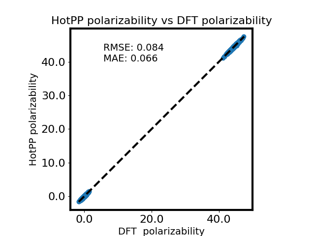
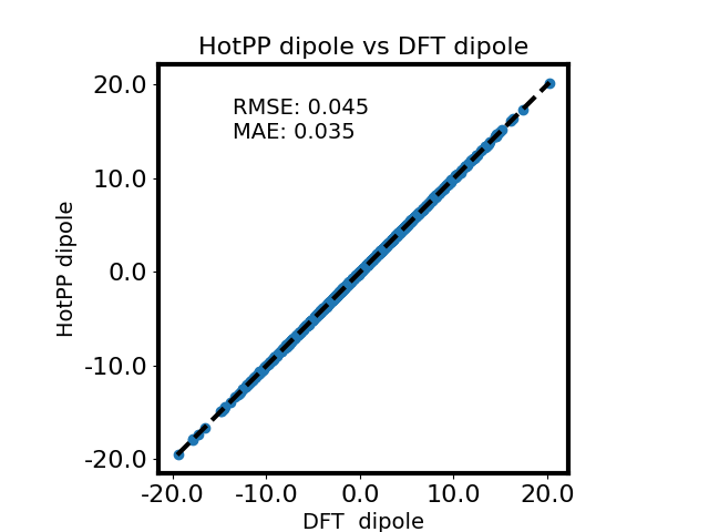
And you can analyze them. To plot them to compare with DFT:
[10]:
! hotpp plot -p polarizability dipole
polarizability: 0.0908 0.0698
   dipole   : 0.0693 0.0515
This command means that we plot polarizability and dipole calculated by HotPP and the target values. And you can see the results:
|
|
|---|---|
|
|
If you need plot peratom polarizability instead of polarizability, just use:
$ hotpp plot -p per_polarizability
Molecule Dynamics
Then we introduce how to calculate infrared and raman spectrum with lammps. First, we freeze the model so you can use it without hotpp being installed.
[24]:
%cd {WORKDIR}
%mkdir lmps
%cd lmps
! hotpp freeze ../dipole/best.pt -o dipole.pt
! hotpp freeze ../polar/best.pt -o polar.pt
/home/gegejun/src/hotpp/examples/water
mkdir: cannot create directory ‘lmps’: File exists
/home/gegejun/src/hotpp/examples/water/lmps
We can get ase-dipole.pt, ase-polar.pt, lammps-dipole.pt, and lammps-polar.pt. As its name, lammps-dipole.pt and lammps-polar.pt are we need. Besides, a machine learning potential is required to run molecular dynamics, and it can be trained as shown in the [carbon] example. Here, we skip this process and directly use the pre-trained force field. In summary, we need:
lmps
|- lammps-dipole.pt      # model to calculate dipole
|- lammps-polar.pt       # model to calculate polarizability
|- lammps-infer.pt       # model to calculate energy, forces, and virials
|- restart.xyz           # initial structure
|- in.lammps             # lammps input file
|- lmp_hotpp             # lammps binary compiled with hotpp
And the lmp_hotpp can be got as shown in the document.
[4]:
! ./lmp_hotpp -in in.lammps
LAMMPS (2 Aug 2023 - Update 1)
OMP_NUM_THREADS environment is not set. Defaulting to 1 thread. (src/lammps-2Aug2023/src/comm.cpp:98)
  using 1 OpenMP thread(s) per MPI task
Reading data file ...
  orthogonal box = (0 0 0) to (13.348493 15.413518 14.532002)
  1 by 1 by 1 MPI processor grid
  reading atoms ...
  288 atoms
  reading velocities ...
  288 velocities
  read_data CPU = 0.003 seconds
The simulations are performed on the GPU
ok
Generated 0 of 1 mixed pair_coeff terms from geometric mixing rule
The simulations are performed on the GPU
ok
The simulations are performed on the GPU
ok
Neighbor list info ...
  update: every = 10 steps, delay = 0 steps, check = no
  max neighbors/atom: 2000, page size: 100000
  master list distance cutoff = 6
  ghost atom cutoff = 6
  binsize = 3, bins = 5 6 5
  3 neighbor lists, perpetual/occasional/extra = 1 2 0
  (1) pair miao, perpetual
      attributes: full, newton on
      pair build: full/bin/atomonly
      stencil: full/bin/3d
      bin: standard
  (2) compute miao/dipole, occasional, copy from (1)
      attributes: full, newton on
      pair build: copy
      stencil: none
      bin: none
  (3) compute miao/polarizability, occasional, copy from (1)
      attributes: full, newton on
      pair build: copy
      stencil: none
      bin: none
Setting up Verlet run ...
  Unit style    : metal
  Current step  : 0
  Time step     : 0.0005
Per MPI rank memory allocation (min/avg/max) = 3.398 | 3.398 | 3.398 Mbytes
   Step         PotEng         KinEng         TotEng          Temp          Press          Volume
         0  -25.274113      10.595795     -14.678317      285.61896      5714.4326      2989.9194
      2000  -24.876068      10.762293     -14.113775      290.10705      5837.1078      2989.9194
      4000  -25.068634      10.552267     -14.516367      284.44561      10893.037      2989.9194
      6000  -24.807093      10.840265     -13.966828      292.20884      5121.4215      2989.9194
      8000  -24.696821      10.775416     -13.921405      290.46078      8179.3193      2989.9194
     10000  -24.577827      10.886911     -13.690916      293.46624      13758.63       2989.9194
     12000  -25.001028      11.466796     -13.534232      309.09753      9750.4965      2989.9194
     14000  -24.072268      11.033265     -13.039002      297.41134      4151.8793      2989.9194
     16000  -24.983761      11.832023     -13.151737      318.94257      7842.389       2989.9194
     18000  -25.091131      12.09712      -12.994011      326.08848      12013.717      2989.9194
     20000  -24.735641      11.603845     -13.131797      312.79181      1327.8405      2989.9194
     22000  -24.224955      11.955183     -12.269772      322.26244      6106.2622      2989.9194
     24000  -24.92952       11.920466     -13.009054      321.32661      4742.5286      2989.9194
     26000  -24.36871       11.703269     -12.665441      315.47187      10279.647      2989.9194
     28000  -23.61507       11.501316     -12.113755      310.02805      6013.8162      2989.9194
     30000  -24.571568      12.66074      -11.910828      341.28134      4684.8707      2989.9194
     32000  -24.174849      12.356578     -11.81827       333.0824       4163.8555      2989.9194
     34000  -23.360071      12.387513     -10.972559      333.91627      11846.909      2989.9194
     36000  -24.550678      14.121505     -10.429173      380.65755      8654.3688      2989.9194
     38000  -23.345896      12.612058     -10.733838      339.96908      8257.0962      2989.9194
     40000  -22.509384      12.357559     -10.151825      333.10883      2826.3801      2989.9194
Loop time of 1968.52 on 1 procs for 40000 steps with 288 atoms

Performance: 0.878 ns/day, 27.341 hours/ns, 20.320 timesteps/s, 5.852 katom-step/s
92.1% CPU use with 1 MPI tasks x 1 OpenMP threads

MPI task timing breakdown:
Section |  min time  |  avg time  |  max time  |%varavg| %total
---------------------------------------------------------------
Pair    | 1273.1     | 1273.1     | 1273.1     |   0.0 | 64.67
Neigh   | 3.8581     | 3.8581     | 3.8581     |   0.0 |  0.20
Comm    | 0.49211    | 0.49211    | 0.49211    |   0.0 |  0.02
Output  | 0.00097652 | 0.00097652 | 0.00097652 |   0.0 |  0.00
Modify  | 690.99     | 690.99     | 690.99     |   0.0 | 35.10
Other   |            | 0.1057     |            |       |  0.01

Nlocal:            288 ave         288 max         288 min
Histogram: 1 0 0 0 0 0 0 0 0 0
Nghost:           1640 ave        1640 max        1640 min
Histogram: 1 0 0 0 0 0 0 0 0 0
Neighs:              0 ave           0 max           0 min
Histogram: 1 0 0 0 0 0 0 0 0 0
FullNghs:        25640 ave       25640 max       25640 min
Histogram: 1 0 0 0 0 0 0 0 0 0

Total # of neighbors = 25640
Ave neighs/atom = 89.027778
Neighbor list builds = 4000
Dangerous builds not checked
Total wall time: 0:32:59
Now we have got dipole.txt and polar.txt, and can calculate IR and Raman by:
[14]:
%cp ../../../tools/spectrum.py .
import numpy as np
from spectrum import load_lmps_dipole, load_lmps_polar, calc_acf_dp, calc_acf_beta, calc_ir, calc_raman, fs
import matplotlib.pyplot as plt

N = 1000
T = 298.15
dt = 1 * fs
w_max = 4000

dipole = load_lmps_dipole("dipole.txt")
acf_dp = calc_acf_dp(dipole, N)
freq, ir = calc_ir(acf_dp, N, T, dt, w_max)
ir = ir / ir.max()

fig = plt.figure(figsize=(12, 7))
fig.patch.set_facecolor('white')
ax = plt.gca()
ax.spines['bottom'].set_linewidth(3)
ax.spines['left'].set_linewidth(3)
ax.spines['right'].set_linewidth(3)
ax.spines['top'].set_linewidth(3)
ax.tick_params(labelsize=16)
ax.set_xlabel('Frequency (cm-1)', fontsize=20)
ax.set_ylabel('IR intensity (arb. units)', fontsize=20)
plt.plot(freq, ir, color='blue', linewidth=3)
plt.savefig("ir.png")
plt.close()

polar = load_lmps_polar("polar.txt")
acf_beta = calc_acf_beta(polar, N)
freq, raman = calc_raman(acf_beta, N, T, dt, w_max)
raman /= raman.max()

fig = plt.figure(figsize=(12, 7))
fig.patch.set_facecolor('white')
ax = plt.gca()
ax.spines['bottom'].set_linewidth(3)
ax.spines['left'].set_linewidth(3)
ax.spines['right'].set_linewidth(3)
ax.spines['top'].set_linewidth(3)
ax.tick_params(labelsize=16)
ax.set_xlabel('Frequency (cm-1)', fontsize=20)
ax.set_ylabel('anisotropic Raman intensity (arb. units)', fontsize=20)
plt.plot(freq, raman, color='blue', linewidth=3)
plt.savefig("raman.png")
plt.close()
And you can see the results: |IR|Raman| |:-:|:-:| ||915150ac436c4cbead025446adf74af9|||6664e28f38034102aabbe07376ac4889||